A formal theory for estimating defeaturing -induced engineering analysis errors

Sankara Hari Gopalakrishnan, Krishnan Suresh

Department of Mechanical Engineering, University of Wisconsin, Madison, WI 53706, United States
Received 13 January 2006; accepted 30 September 2006

Abstract

Defeaturing is a popular CAD/CAE simplification technique that suppresses ‘small or irrelevant features’ within a CAD model to speed-up downstream processes such as finite element analysis. Unfortunately, defeaturing inevitably leads to analysis errors that are not easily quantifiable within the current theoretical framework.

In this paper, we provide a rigorous theory for swiftly computing such defeaturing -induced engineering analysis errors. In particular, we focus on problems where the features being suppressed are cutouts of arbitrary shape and size within the body. The proposed theory exploits the adjoint formulation of boundary value problems to arrive at strict bounds on defeaturing induced analysis errors. The theory is illustrated through numerical examples.

Keywords: Defeaturing; Engineering analysis; Error estimation; CAD/CAE

1. Introduction

Mechanical artifacts typically contain numerous geometric features. However, not all features are critical during engineering analysis. Irrelevant features are often suppressed or ‘defeatured’, prior to analysis, leading to increased automation and computational speed-up.

For example, consider a brake rotor illustrated in Fig. 1(a). The rotor contains over 50 distinct ‘features’, but not all of these are relevant during, say, a thermal analysis. A defeatured brake rotor is illustrated in Fig. 1(b). While the finite element analysis of the full-featured model in Fig. 1(a) required over 150,000 degrees of freedom, the defeatured model in Fig. 1(b) required <25,000 DOF, leading to a significant computational speed-up.

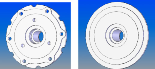
Fig. 1. (a) A brake rotor and                 (b) its defeatured version.

Besides an improvement in speed, there is usually an increased level of automation in that it is easier to automate finite element mesh generation of a defeatured component [1,2]. Memory requirements also decrease, while condition number of the discretized system improves;the latter plays an important role in iterative linear system solvers [3].

Defeaturing, however, invariably results in an unknown ‘perturbation’ of the underlying field. The perturbation may be ‘small and localized’ or ‘large and spread-out’, depending on various factors. For example, in a thermal problem, suppose one deletes a feature; the perturbation is localized provided: (1) the net heat flux on the boundary of the feature is zero, and (2) no new heat sources are created when the feature is suppressed; see [4] for exceptions to these rules. Physical features that exhibit this property are called self-equilibrating [5]. Similarly results exist for structural problems.

From a defeaturing perspective, such self-equilibrating features are not of concern if the features are far from the region of interest. However, one must be cautious if the features are close to the regions of interest.

On the other hand, non-self-equilibrating features are of even higher concern. Their suppression can theoretically be felt everywhere within the system, and can thus pose a major challenge during analysis.

Currently, there are no systematic procedures for estimating the potential impact of defeaturing in either of the above two cases. One must rely on engineering judgment and experience.

In this paper, we develop a theory to estimate the impact of defeaturing on engineering analysis in an automated fashion. In particular, we focus on problems where the features being suppressed are cutouts of arbitrary shape and size within the body. Two mathematical concepts, namely adjoint formulation and monotonicity analysis, are combined into a unifying theory to address both self-equilibrating and non-self-equilibrating features. Numerical examples involving 2nd order scalar partial differential equations are provided to substantiate the theory.

The remainder of the paper is organized as follows. In Section 2, we summarize prior work on defeaturing. In Section 3, we address defeaturing induced analysis errors, and discuss the proposed methodology. Results from numerical experiments are provided in Section 4. A by-product of the proposed work on rapid design exploration is discussed in Section 5. Finally, conclusions and open issues are discussed in Section 6.

2. Prior work

The defeaturing process can be categorized into three phases:

Identification: what features should one suppress?

Suppression: how does one suppress the feature in an automated and geometrically consistent manner?

Analysis: what is the consequence of the suppression?

The first phase has received extensive attention in the literature. For example, the size and relative location of a feature is often used as a metric in identification [2,6]. In addition, physically meaningful ‘mechanical criterion/heuristics’ have also been proposed for identifying such features [1,7].

To automate the geometric process of defeaturing, the authors in [8] develop a set of geometric rules, while the authors in [9] use face clustering strategy and the authors in [10] use plane splitting techniques. Indeed, automated geometric defeaturing has matured to a point where commercial defeaturing /healing packages are now available [11,12]. But note that these commercial packages provide a purely geometric solution to the problem... they must be used with care since there are no guarantees on the ensuing analysis errors. In addition, open geometric issues remain and are being addressed [13].

The focus of this paper is on the third phase, namely, post defeaturing analysis, i.e., to develop a systematic methodology through which defeaturing -induced errors can be computed. We should mention here the related work on reanalysis. The objective of reanalysis is to swiftly compute the response of a modified system by using previous simulations. One of the key developments in reanalysis is the famous Sherman–Morrison and Woodbury formula [14] that allows the swift computation of the inverse of a perturbed stiffness matrix; other variations of this based on Krylov subspace techniques have been proposed [15–17]. Such reanalysis techniques are particularly effective when the objective is to analyze two designs that share similar mesh structure, and stiffness matrices. Unfortunately, the process of 几何分析 can result in a dramatic change in the mesh structure and stiffness matrices, making reanalysis techniques less relevant.

A related problem that is not addressed in this paper is that of local–global analysis [13], where the objective is to solve the local field around the defeatured region after the global defeatured problem has been solved. An implicit assumption in local–global analysis is that the feature being suppressed is self-equilibrating.

3. Proposed methodology

3.1. Problem statement

We restrict our attention in this paper to engineering problems involving a scalar field u governed by a generic 2nd order partial differential equation (PDE):

A large class of engineering problems, such as thermal, fluid and magneto-static problems, may be reduced to the above form.

As an illustrative example, consider a thermal problem over the 2-D heat-block assembly Ω illustrated in Fig. 2.

The assembly receives heat Q from a coil placed beneath the region identified as Ωcoil. A semiconductor device is seated at Ωdevice. The two regions belong to Ω and have the same material properties as the rest of Ω. In the ensuing discussion, a quantity of particular interest will be the weighted temperature Tdevice within Ωdevice (see Eq. (2) below). A slot, identified as Ωslot in Fig. 2, will be suppressed, and its effect on Tdevice will be studied. The boundary of the slot will be denoted by Γslot while the rest of the boundary will be denoted by Γ. The boundary temperature on Γ is assumed to be zero. Two possible boundary conditions on Γslot are considered: (a) fixed heat source, i.e., (-krT).ˆn = q, or (b) fixed temperature, i.e., T = Tslot. The two cases will lead to two different results for defeaturing induced error estimation.

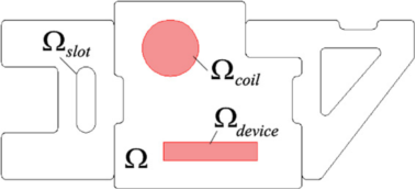
Fig. 2. A 2-D heat block assembly.

Formally,let T (x, y) be the unknown temperature field and k the thermal conductivity. Then, the thermal problem may be stated through the Poisson equation [18]:

Given the field T (x, y), the quantity of interest is:

where H(x, y) is some weighting kernel. Now consider the defeatured problem where the slot is suppressed prior to analysis, resulting in the simplified geometry illustrated in Fig. 3.

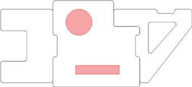
Fig. 3. A defeatured 2-D heat block assembly.

We now have a different boundary value problem, governing a different scalar field t (x, y):

Observe that the slot boundary condition for t (x, y) has disappeared since the slot does not exist any more…a crucial change!

The problem addressed here is:

Given tdevice and the field t (x, y), estimate Tdevice without explicitly solving Eq. (1).

This is a non-trivial problem; to the best of our knowledge,it has not been addressed in the literature. In this paper, we will derive upper and lower bounds for Tdevice. These bounds are explicitly captured in Lemmas 3.4 and 3.6. For the remainder of this section, we will develop the essential concepts and theory to establish these two lemmas. It is worth noting that there are no restrictions placed on the location of the slot with respect to the device or the heat source, provided it does not overlap with either. The upper and lower bounds on Tdevice will however depend on their relative locations.

3.2. Adjoint methods

The first concept that we would need is that of adjoint formulation. The application of adjoint arguments towards differential and integral equations has a long and distinguished history [19,20], including its applications in control theory [21],shape optimization [22], topology optimization, etc.; see [23] for an overview.We summarize below concepts essential to this paper.

Associated with the problem summarized by Eqs. (3) and (4), one can define an adjoint problem governing an adjoint variable denoted by t_(x, y) that must satisfy the following equation [23]: (See Appendix A for the derivation.)

The adjoint field t_(x, y) is essentially a ‘sensitivity map’ of the desired quantity, namely the weighted device temperature to the applied heat source. Observe that solving the adjoint problem is only as complex as the primal problem; the governing equations are identical; such problems are called self-adjoint. Most engineering problems of practical interest are self-adjoint, making it easy to compute primal and adjoint fields without doubling the computational effort.

For the defeatured problem on hand, the adjoint field plays a critical role as the following lemma summarizes:

Lemma 3.1. The difference between the unknown and known device temperature, i.e., (Tdevice − tdevice), can be reduced to the following boundary integral over the defeatured slot:

Two points are worth noting in the above lemma:

1. The integral only involves the slot boundary Гslot; this is encouraging … perhaps, errors can be computed by processing information just over the feature being suppressed.

2. The right hand side however involves the unknown field T (x, y) of the full-featured problem. In particular, the first term involves the difference in the normal gradients, i.e.,involves [−k(T − t)]. ˆn; this is a known quantity if Neumann boundary conditions [−kT ]. ˆn are prescribed over the slot since [−kt]. ˆn can be evaluated, but unknown if Dirichlet conditions are prescribed. On the other hand,the second term involves the difference in the two fields,i.e., involves (T − t); this is a known quantity if Dirichlet boundary conditions T are prescribed over the slot since t can be evaluated, but unknown if Neumann conditions are prescribed. Thus, in both cases, one of the two terms gets ‘evaluated’. The next lemma exploits this observation.

Lemma 3.2. The difference (Tdevice − tdevice) satisfies the inequalities

Unfortunately, that is how far one can go with adjoint techniques; one cannot entirely eliminate the unknown field T (x, y) from the right hand side using adjoint techniques. In order to eliminate T (x, y) we turn our attention to monotonicity analysis.

3.3. Monotonicity analysis

Monotonicity analysis was established by mathematicians during the 19th and early part of 20th century to establish the existence of solutions to various boundary value problems [24].For example, a monotonicity theorem in [25] states:

“On adding geometrical constraints to a structural problem,the mean displacement over (certain) boundaries does not decrease”.

Observe that the above theorem provides a qualitative measure on solutions to boundary value problems.

Later on, prior to the ‘computational era’, the same theorems were used by engineers to get quick upper or lower bounds to challenging problems by reducing a complex problem to simpler ones [25]. Of course, on the advent of the computer, such methods and theorems took a back-seat since a direct numerical solution of fairly complex problems became feasible.However, in the present context of defeaturing, we show that these theorems take on a more powerful role, especially when used in conjunction with adjoint theory.

We will now exploit certain monotonicity theorems to eliminate T (x, y) from the above lemma. Observe in the previous lemma that the right hand side involves the difference between the known and unknown fields, i.e., T (x, y) − t (x, y). Let us therefore define a field e(x, y) over the region  as:

e(x, y) = T (x, y) − t (x, y) in .

Note that since  excludes the slot, T (x, y) and t (x, y) are both well defined in , and so is e(x, y). In fact, from Eqs. (1) and (3) we can deduce that e(x, y) formally satisfies the boundary value problem:

Solving the above problem is computationally equivalent to solving the full-featured problem of Eq. (1). But, if we could compute the field e(x, y) and its normal gradient over the slot,in an efficient manner, then (Tdevice − tdevice) can be evaluated from the previous lemma. To evaluate e(x, y) efficiently, we now consider two possible cases (a) and (b) in the above equation.

Case (a) Neumann boundary condition over slot

First, consider the case when the slot was originally assigned a Neumann boundary condition. In order to estimate e(x, y),consider the following exterior Neumann problem:

The above exterior Neumann problem is computationally inexpensive to solve since it depends only on the slot, and not on the domain . Classic boundary integral/boundary element methods can be used [26]. The key then is to relate the computed field e1(x, y) and the unknown field e(x, y) through the following lemma.Lemma 3.3. The two fields e1(x, y) and e(x, y) satisfy the following monotonicity relationship:

Proof. Proof exploits triangle inequality.

Piecing it all together, we have the following conclusive lemma.

Lemma 3.4. The unknown device temperature Tdevice, when the slot has Neumann boundary conditions prescribed, is bounded by the following limits whose computation only requires: (1) the primal and adjoint fields t and t_ associated with the defeatured domain, and (2) the solution e1 to an exterior Neumann problem involving the slot:

Proof. Follows from the above lemmas. _

Observe that the two bounds on the right hand sides are independent of the unknown field T (x, y).

Case (b) Dirichlet boundary condition over slot

Let us now consider the case when the slot is maintained at a fixed temperature Tslot. Consider any domain − that is contained by the domain  that contains the slot. Define a field e−(x, y) in − that satisfies:

We now establish a result relating e−(x, y) and e(x, y).

Lemma 3.5.

Note that the problem stated in Eq. (7) is computationally less intensive to solve. This leads us to the final result.

Lemma 3.6. The unknown device temperature Tdevice, when the slot has Dirichlet boundary conditions prescribed, is bounded by the following limits whose computation only requires: (1) the primal and adjoint fields t and t_ associated with the defeatured domain, and (2) the solution e− to a collapsed boundary problem surrounding the slot:

Proof. Follows from the above lemmas.

Observe again that the two bounds are independent of the unknown field T (x, y).

4. Numerical examples

We illustrate the theory developed in the previous section through numerical examples.

Let k = 5W/m−C, Q = 10 W/m3 and H = .

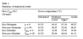
Table 1 shows the numerical results for different slot boundary conditions. The first device temperature column is the common temperature for all defeatured models (it does not depend on the slot boundary conditions since the slot was defeatured).The next two columns are the upper and lower bounds predicted by Lemmas 3.4 and 3.6. The last column is the actual device temperature obtained from the full-featured model (prior to defeaturing),and is shown here for comparison purposes.In all the cases, we can see that the last column lies between the 2nd and 3rd column, i.e.T Tdevice T

Observe that the range predicted for the zero Dirichlet condition is much wider than that for the insulated-slot scenario. The difference lies in the fact that in the first example,a zero Neumann boundary condition on the slot resulted in a self-equilibrating feature, and hence its effect on the device was minimal. On the other hand, a Dirichlet boundary condition on the slot results in a non-self-equilibrating feature whose deletion can result in a large change in the device temperature.

Observe however that the predicted range for a fixed nonzero slot temperature of 20 _C is narrower than that for the zerotemperature scenario. This can be attributed to the fact the slot temperature is closer to the device temperature and therefore its deletion has less of an impact.

Indeed, one can easily compute the upper and lower bounds different Dirichlet conditions for the slot. Fig. 4 illustrates the variation of the actual device temperature and the computed bounds as a function of the slot temperature.

Observe that the theory correctly predicts the upper and lower limits of the actual device temperature. Further, the limits are tightest when the slot-temperature is approximately equal to the device temperature, as expected.

5. Rapid analysis of design scenarios

We consider now a broader impact of the proposed theory in analyzing “what-if” design scenarios. Consider the design shown in Fig. 5 that now consists of two devices with a single heat source.As expected, the two devices will not be at the same average temperature. The device on the left will be at a higher temperature due to its relative proximity to the heat source.

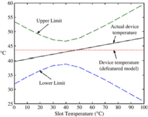
Fig. 4. Estimated bounds versus slot temperature

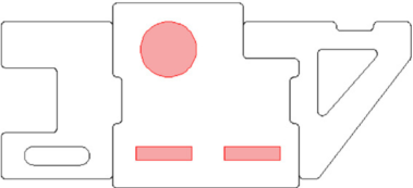
Fig. 5. Dual device heat block.

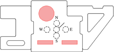
Fig. 6. Possible locations for a correcting feature.

Consider the scenario where one wishes to correct the imbalance by adding a small hole of fixed diameter; five possible locations are illustrated in Fig. 6. An optimal position has to be chosen such that the difference in the average temperatures of the two regions is minimized.

A brute force strategy would be to carry out the finite element analysis for each configuration . . . a time consuming process. An alternate strategy is to treat the hole as a ‘feature’ and study its impact as a post-processing step. In other words,this is a special case of ‘defeaturing’, and the proposed methodology applies equally to the current scenario.

We can solve the primal and adjoint problems for the original configuration (without the hole) and use the theory developed in the previous sections to study the effect of adding the hole at each position on our objective. The objective is to minimize the difference in the average temperature of the two devices.

Table 2 summarizes the bounds predicted using this theory, and the actual values.

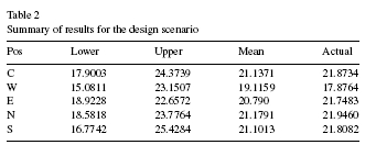
From the table, it can be seen that the location W is the optimal location since it gives the lowest mean value for the desired objective function, as expected.