|
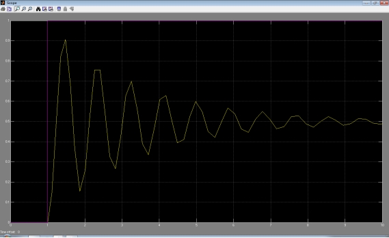
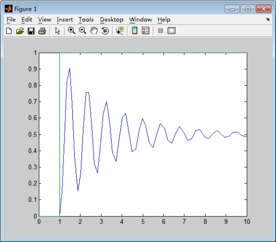
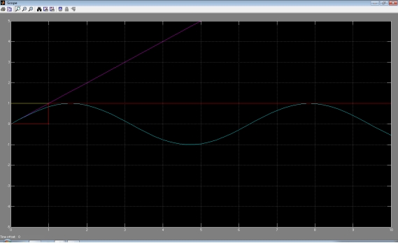
[1] 建立如图1所示系统结构的Simulink模型,并用示波器(Scope)观测其单位阶跃和斜坡响应曲线。
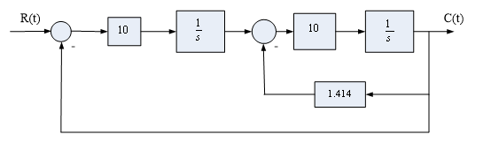 图 1 图 1
a. 输入为阶跃信号时:
模型为
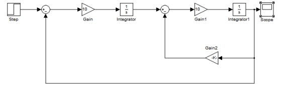
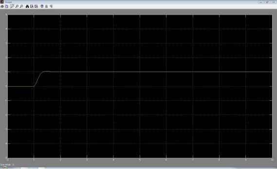
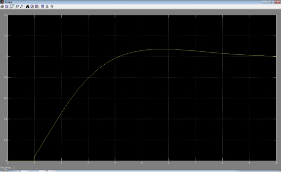
响应曲线:
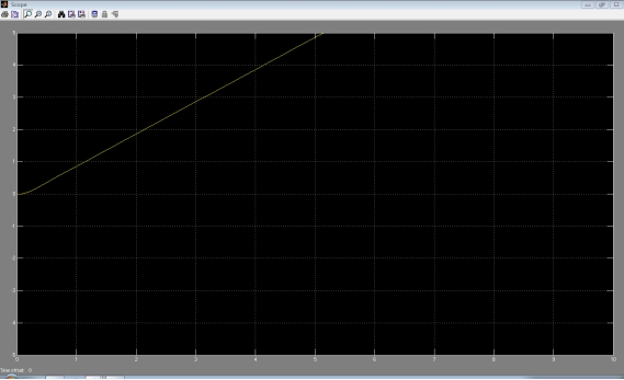
b. 输入为斜坡信号时:
模型为
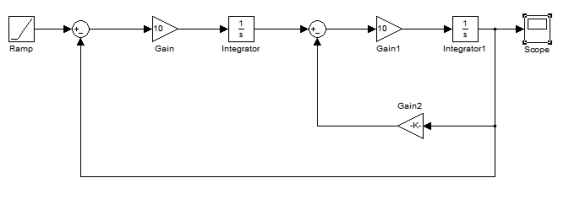
响应曲线为:
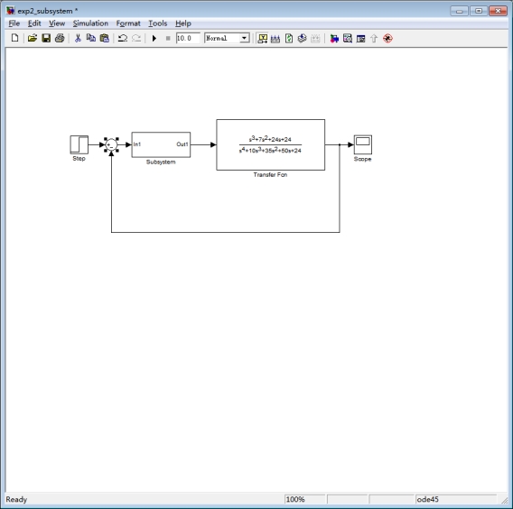
[2] 建立如图2所示PID控制系统的Simulink模型,对系统进行单位阶跃响应仿真,用plot函数绘制出响应曲线。其中 =10, =10, =3, =3, =2。要求PID部分用subsystem实现,参数 =2。要求PID部分用subsystem实现,参数 、 、 、 、 通过subsystem参数输入来实现。 通过subsystem参数输入来实现。
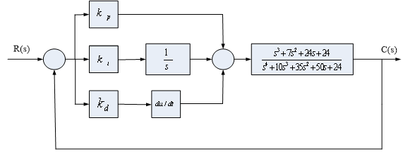 图 2 图 2
模型为:
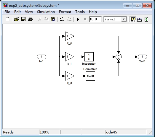
Subsystem:
输出曲线:
用plot 画图:
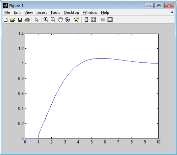
[3] 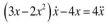 建求解非线性微分方程 的数值解并绘制函数的波形(x与 建求解非线性微分方程 的数值解并绘制函数的波形(x与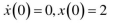 x'的波形),其初始值为: x'的波形),其初始值为:
模型为
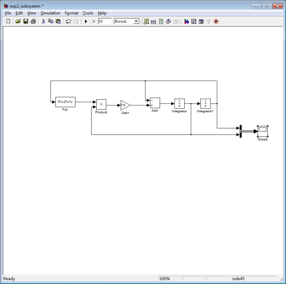
输出响应曲线:
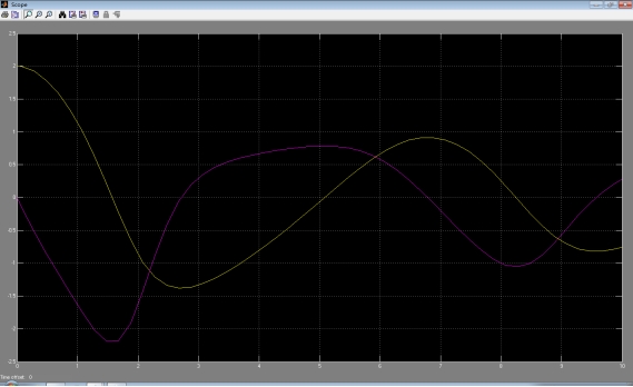
[4] 建立如图4所示非线性控制系统的Simulink模型并仿真,用示波器观测c(t)值,并画出其响应曲线。
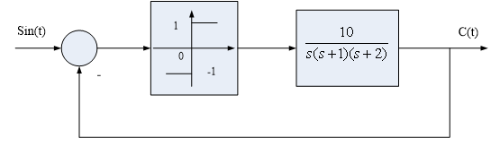 图 4 图 4
模型为:
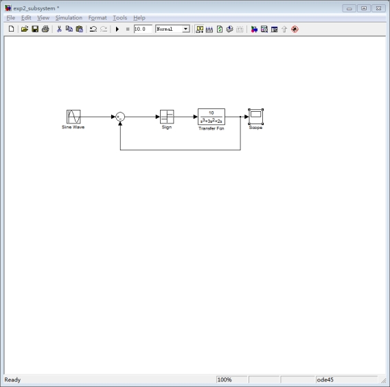
输出响应曲线为:
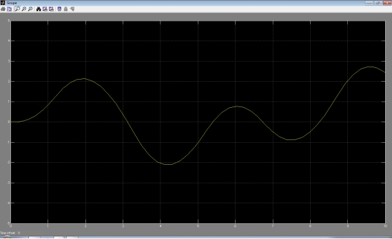
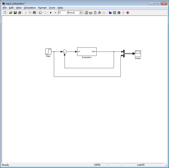
[5] 图5所示为简化的飞行控制系统、试建立此动态系统的simulink模型并进行简单的仿真分析。其中, ,系统输入input为单位阶跃曲线, ,系统输入input为单位阶跃曲线, 。 。
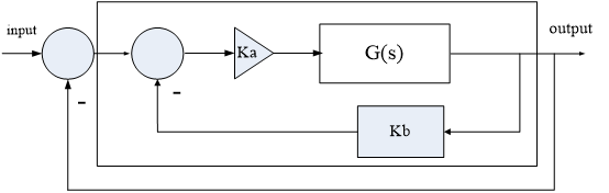
图5
具体要求如下:
(1)采用自顶向下的设计思路。
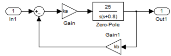
(2)对虚线框中的控制器采用子系统技术。
(3)用同一示波器显示输入信号input与输出信号output。
(4)输出数据output到MATLAB工作空间,并绘制图形。
模型为:
Subsystem:
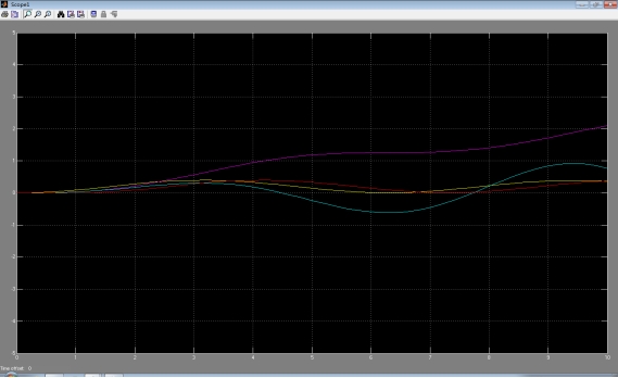
输出响应为:
用plot画图:
[6] 图6所示为弹簧―质量―阻尼器机械位移系统。请建立此动态系统的Simulink仿真模型,然后分析系统在外力F(t)作用下的系统响应(即质量块的位移y(t))。其中质量块质量m=5kg,阻尼器的阻尼系数f=0.5,弹簧的弹性系数K=5;并且质量块的初始位移与初始速度均为0。
说明:外力F(t)由用户自己定义,目的是使用户对系统在不同作用下的性能有更多的了解。
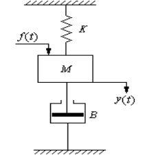
图6 弹簧-质量-阻尼器机械位移系统示意图
提示:
(1)首先根据牛顿运动定律建立系统的动态方程,如下式所示:

(2)由于质量块的位移 未知,故在建立系统模型时.使用积分模块Integrator对位移的微分进行积分以获得位移 未知,故在建立系统模型时.使用积分模块Integrator对位移的微分进行积分以获得位移 ,且积分器初估值均为0。 ,且积分器初估值均为0。
为建立系统模型.将系统动态方程转化为如下的形式:

然后以此式为核心建立系统模型。
四种输入:
输出响应曲线:
|
